Article
Escobari and Hoover’s “Difference Estimates” Are Driven by Geography — Not by “Fraud”

Article
This is the eighth in a series of blog posts addressing a report by Diego Escobari and Gary Hoover covering the 2019 presidential election in Bolivia. Their conclusions do not hold up to scrutiny, as we observe in our report Nickels Before Dimes. Here, we expand upon various claims and conclusions that Escobari and Hoover make in their paper. Links to other posts: part one, part two, part three, part four, part five, part six, part seven, and part nine.
In the previous post, we investigated the confounding effects of rurality and socioeconomic status on a naive estimate of fraud. We noted that if we could divide polling stations into groups such that the confounding effects do not vary within each group, then we may begin to disentangle the effects of, say, Internet connectivity, on whether a station was included in the TSE announcement.
The most obvious way to manage such factors is to assume that voters within small geographic areas are effectively indistinguishable. Of course, the smaller the geographic area, the more truth there will be in this assumption. To a first approximation, we would expect voters of the same precinct to have more similar socioeconomic status or rurality than voters at different precincts, even within the same municipality. At least, we may hope.
Consider column 4 of Escobari and Hoover’s difference estimates. There, the polling stations are grouped by municipality. In practice, this meant performing exactly the same analysis as before, but only after eliminating the average differences in vote margins across municipalities. Importantly, the adjustment comes at the municipality level so that differences between polling stations of the same municipality are preserved. Because the averages depend on the weighting scheme, the adjustments will be different if we take into account the number of valid votes at each polling station.
In Figure 1, we see the unadjusted and (weighted) adjustments for polling stations at two municipalities: New York (United States) and Acasio (Potosí). On the left, we see that New York went heavily for Mesa, while Acasio greatly favored Morales. On the right, we have adjusted the margins to take into account only the differences across municipalities.
Figure 1
Official and Municipality-Adjusted Results in New York and Acasio
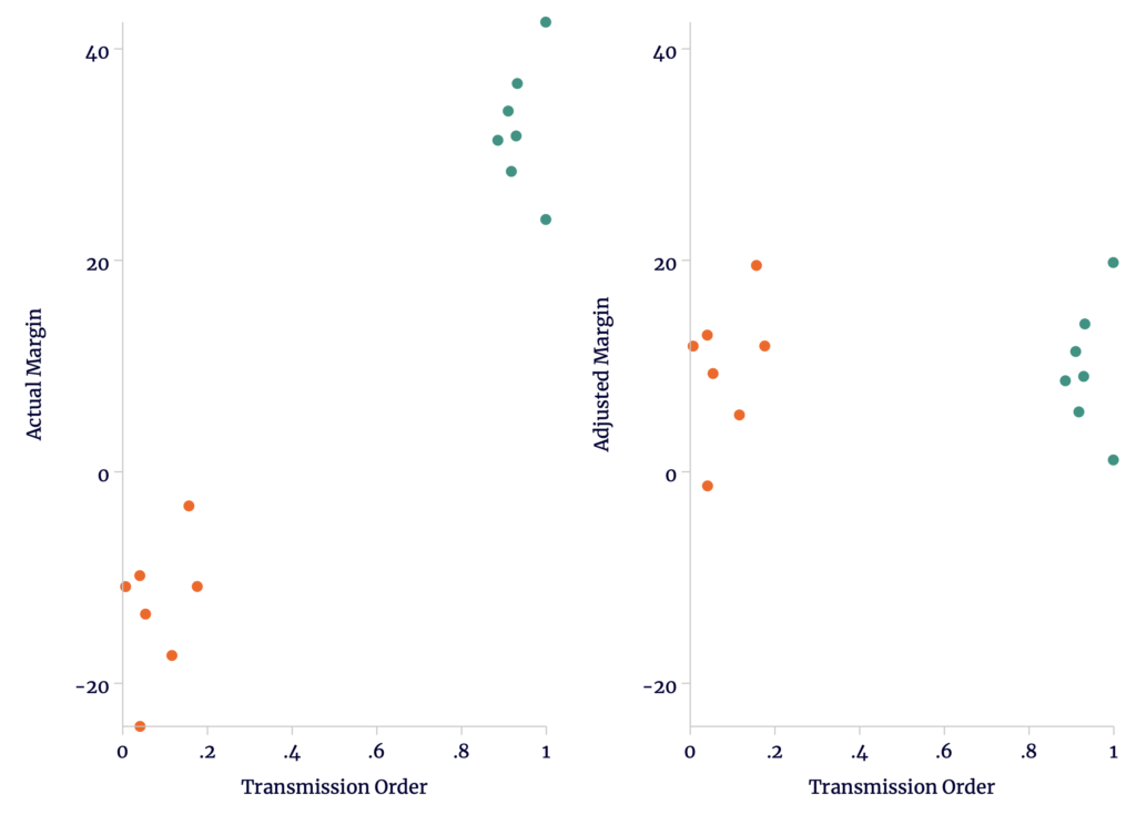
Sources: TSE and author’s calculations.
In Figure 2, we see how applying the adjustment to all municipalities affects the overall trend. We see that municipality explains most, but not all of the trend in support across ARRIVAL.
Figure 2
Official and Municipality-Adjusted Trends in Vote Margin
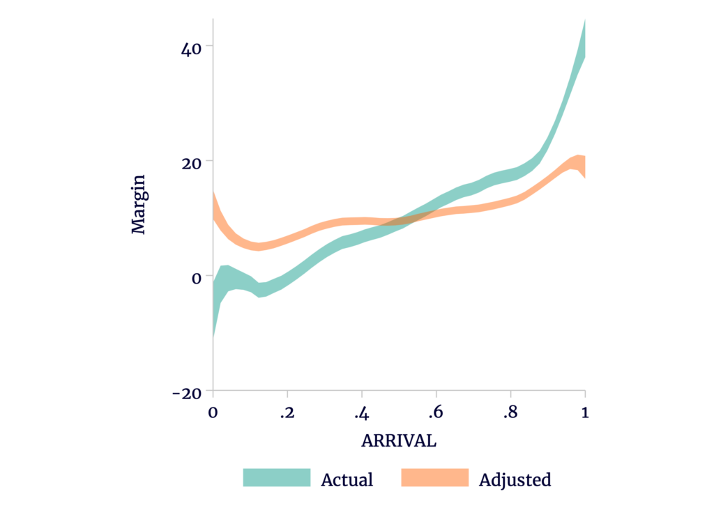
Sources: TSE and author’s calculations.
Our replication and corrections to the municipality-adjusted results are presented alongside their reported results in Table 1.
Table 1
Replication and Reanalyses of Escobari and Hoover’s Municipality-Adjusted Difference Model
| As Published | Replication | Correct Voters | Weighted | |
|---|---|---|---|---|
| (1) | (2) | (3) | (4) | |
| Variable | ||||
| SHUTDOWN | 7.243 (0.437) | 7.243 (0.437) | 7.214 (0.436) | 7.766 (0.447) |
| Constant | 11.28 (0.162) | 11.28 (0.162) | 11.31 (0.162) | 9.32 (0.166) |
| Observations | 34,529 | 34,529 | 34,551 | 34,551 |
| R2 | 0.640 | 0.640 | 0.640 | 0.627 |
Sources: TSE and author’s calculations.
Due to the way that the municipality adjustments (the “fixed effects”) are identified in this particular model, the coefficients are harder to interpret, even when the polling stations are weighted by size. However, when weighted, the mean margin still matches the data: 9.32+0.16 x 7.7766 = 10.56, where 16 percent of votes were excluded from the TSE announcement. More importantly, the effect of the SHUTDOWN is greatly reduced. More than half of the measured effect was coming from differences in municipalityrather than being verified late in the count. This offers considerable evidence that the problem of nickels before dimes is a serious issue that must be completely accounted for when estimating fraud.
As we shrink the group size, the differences between polling stations within each group also narrow. Correspondingly, there is less variation within each group left to explain by exclusion from the TSE announcement. The more we account for confounding factors, the more the SHUTDOWN effect shrinks. The smallest practical unit we may employ is the precinct.
In Figure 3, we see that precincts account for the overall trend almost entirely. Very little is left in the adjusted results.
Figure 3
Official and Precinct-Adjusted Trends in Vote Margin
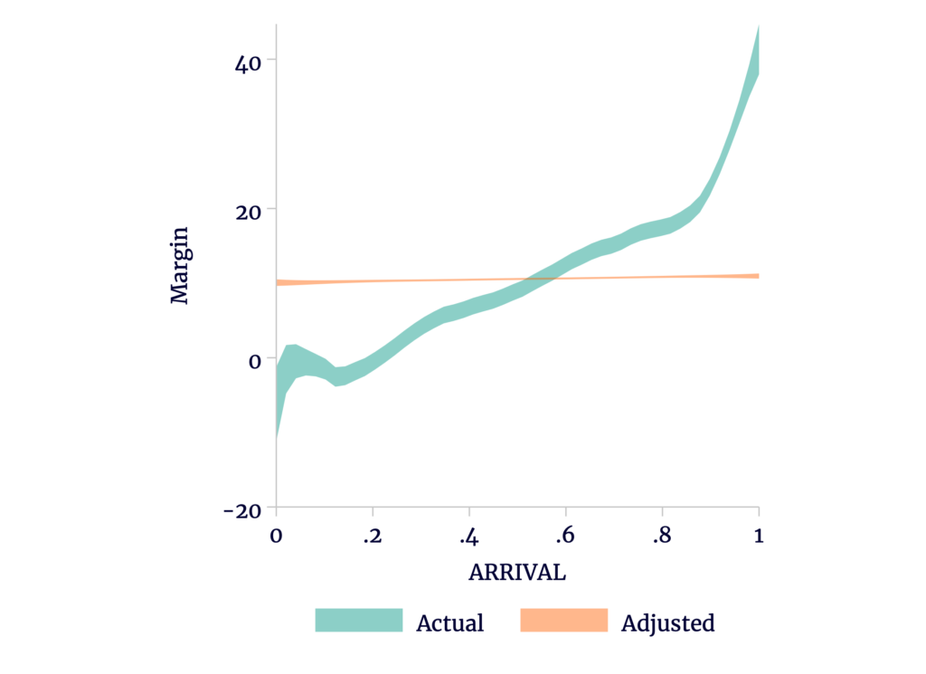
Sources: TSE and author’s calculations.
Table 2
Replication and Reanalyses of Escobari and Hoover’s Precinct-Adjusted Difference Model
| As Published | Replication | Correct Voters | Weighted | |
|---|---|---|---|---|
| (1) | (2) | (3) | (4) | |
| Variable | ||||
| SHUTDOWN | 0.365 (0.194) | 0.377 (0.194) | 0.360 (0.193) | 0.287 (0.192) |
| Constant | 12.39 (0.0631) | 12.39 (0.0631) | 12.41 (0.0630) | 10.52 (0.0632) |
| Observations | 34,529 | 34,529 | 34,551 | 34,551 |
| R2 | 0.958 | 0.958 | 0.958 | 0.958 |
Sources: TSE and author’s calculations.
Rather than an increase of 16 percentage points, we see that on average in a given split precinct, the excluded polling stations favored Morales by only an additional 0.3 percentage points — or about 3,000 net votes. This difference is far from politically significant, with the model otherwise explaining all but 0.046 percentage points of Morales’s final margin.
Again, this doesn’t mean that the 3,000 votes amounted to fraud; it means that we have yet to offer any alternative explanation for the otherwise unexpected difference. For example, if surname is associated with both support for Morales and delays in reporting, the difference could be accounted for there. According to Escobari and Hoover, voters with surnames starting with “Z” voted more strongly in favor of Mesa when compared to others. Perhaps such surnames are associated with a particular socioeconomic status. In any case, coming at the end of the alphabet, “Z” voters voters are assigned to the highest-numbered polling stations in a given precinct, and therefore tend to report early (subject to the “small-station” effect discussed in post #3). Thus, we observe a bias in polling stations with opposition-heavy “Z” voters reporting disproportionately early and so more likely to be included in the TSE announcement. In turn, this would cause us to underestimate Morales’s support in polling stations excluded from the announcement. Worse, Escobari and Hoover do not weigh polling stations by the number of voters, so smaller “Z” surname-heavy stations have oversized impacts on the analysis, exaggerating the difference.[1]
We do not explore whether the 3,000 votes may be accounted for in this manner or, alternatively, if other explanations (potentially including fraud) are required. However, even if we assume that the entire 3,000-vote difference came from fraud, this only would knock Morales’s margin down to 10.52 percentage points — not nearly enough to change the outcome of the election.
This has two important takeaways. First, geography has the capacity to explain much of the increase in Morales’s support. Even if we assume the worst interpretation of the results, the increase in support officially reported for Morales among the late polling stations in split precincts is very small. Second, because 84 percent of the late polling stations came from these split precincts, there is little room left for politically relevant fraud. Escobari and Hoover’s 16.26 percentage points do not form a credible estimate of fraud in the late polling stations.
To illustrate, note that Escobari and Hoover pin their fraud estimate at just under 160,000 votes. If we generously quadruple the number of unexpected votes coming from late polling stations in split precincts (12,000 instead of only 3,000), this leaves 148,000 “fraudulent” votes among the 153,890 valid votes cast in the late precincts. In other words, to reconcile with Escobari and Hoover’s estimate of 16.26 percentage points (see previous post), the late polling stations — officially reported as having supported Morales by more than 50 percentage points — actually supported Mesa by about 45 percentage points.
This would be not only a shockingly obvious level of manipulation, it would need to be vote manipulation in polling stations overwhelmingly in favor of Mesa. These would be stations where most jurors would be Mesa voters, where Mesa voters would witness ballot counting, and where a CC (Mesa’s party) representative likely would be present and offered a copy of the acta as a security measure. It would make no sense for Morales-friendly fraud to take place at these polling stations. And if forged actas were later offered as substitutes, where are the copies of the originals? The OAS audit report indicates that its audit team compared official actas with copies it obtained, but the report did not mention any instances of numerical discrepancy.
Absent any credible way that this level of vote manipulation could have been carried out, we fall back on a much more plausible explanation: Escobari and Hoover’s interpretation of their results as a measure of fraud is incorrect.
In the next post, we will begin to explore approaches to disentangle the effect of geography from that of possible precinct-level manipulations.
[1] On the other hand, they report that “Y” voters favored Morales, so in many areas the effect may be reversed.