Article
The Parable of Nickels Before Dimes: A Tale of Two Roommates

Article
This is the second in a series of blog posts addressing a report by Diego Escobari and Gary Hoover covering the 2019 presidential election in Bolivia. Their conclusions do not hold up to scrutiny, as we observe in our report Nickels Before Dimes. Here, we expand upon various claims and conclusions that Escobari and Hoover make in their paper. Links to other posts: part one, part three, part four, part five, part six, part seven, part eight, and part nine.
Alex reminds Blake, “Don’t forget it’s my night to pick.”
“We’re a dollar thirty short,” says Blake. “We can’t afford your fancy pizza. Let’s just go get those awesome sandwiches from the corner store.”
“A dollar thirty?” responds Alex, “You really don’t want pizza, do you? Go check the swear jar. There’s enough there.”
“Alex, there’s only twenty coins in here. That’s not enough.” Blake starts pulling out coins, one by one. Ten coins in, they hold eight nickels and two dimes. “Sorry, Alex, I’m halfway done counting, but we only have 60 cents. I’m going downstairs for sandwiches.”
By the time Blake returns with their sandwiches, Alex is livid. “I counted the rest of the jar. A dollar thirty more for pizza, and we have a dollar fifty. I told you there was enough money. I can’t believe you’d lie rather than get pizza.”
“I can’t believe you’d accuse me of lying, Alex. The first half of the jar came to 60 cents. That’s only a dollar twenty total. I don’t know where you got the extra thirty cents, but it wasn’t from the jar.”
The phone rings, and Alex picks up. It’s their friend Charlie calling about meeting up this coming weekend. Alex, exasperated, tells the story of what happened. Charlie frowns. “Y’all will be much happier if you sort out some issues with your dinner decisions. But let’s think this through. Just because the first ten coins were eight nickels and two dimes doesn’t mean the other ten counts were eight nickels and two dimes. Even if Blake had drawn at random from a jar of ten nickels and ten dimes, there is a one in 87 chance that eight of the first ten would be nickels.”
“See!” Blake retorts, “That’s not very likely, so Alex added money to the jar.”
Charlie takes a deep breath. “One in 87 is not very likely, but not at all impossible. It could just have been bad luck. Yet there is a more innocuous explanation. Nickels are bigger than dimes. If Blake simply drew the first coin they touched, it would more likely be a nickel. Depending on how Blake happened to draw the coins the odds could have been one in eight, or maybe one in three. They may not have realized the bias in selecting nickels before dimes.
“It doesn’t matter if Blake drew nickels before dimes deliberately or unwittingly. Deciding halfway through the count that there wasn’t enough money and buying sandwiches was premature.”
What is the point of this parable in terms of alleged election fraud? When counting votes in an election, the only thing that matters is the final count. So long as we count all the votes, the order in which we count is unimportant. We could count all the votes for candidate A first, then those for candidate B. Ordering the count in this manner, however, the results of any partial count are misleading.
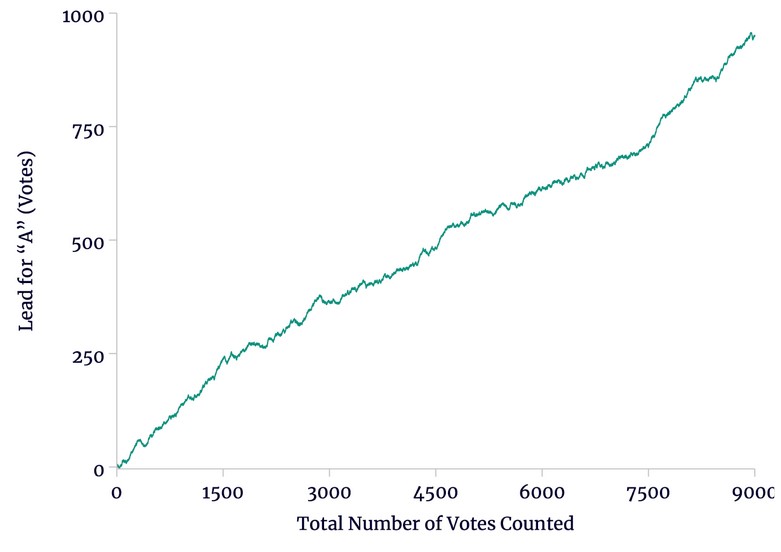
If we are to weigh the risk of being misled by a bias in counting, we must consider what a biased count might look like. In Figure 1, we see how candidate A’s lead might increase as a count progresses. In this example, there is no bias; the deviations from a straight line is pure chance. At the end of the count candidate A has won by 950 votes out of 9,000 total.
Figure 1
An Example Count with No Bias
Source: author’s calculations.
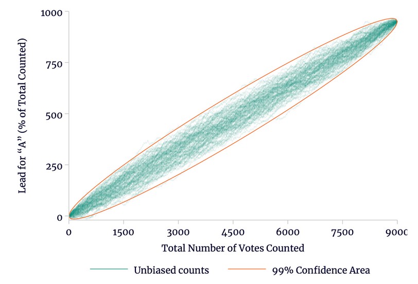
In Figure 2, we see 100 different counts. Note that the votes are exactly the same in all 100 counts, but the order of ballots in each count is different. Again, there is no bias in the selection of votes, so at the end of all 100 counts candidate A has won by exactly the same 950 votes.
Figure 2
One Hundred Unbiased Counts
Source: author’s calculations.
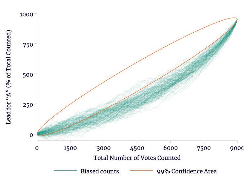
However, if we introduce a slight bias, the count starts looking very different. In Figure 3, we add a biased count: of the remaining votes, any given vote for B is 14 percent more likely to be counted next when compared to any given vote for A. Because there are more votes for A than B, however, the first vote counted will be for A 52 percent of the time. Candidate A still wins by 950 votes once the count is completed. However, early in the count, the lead grows slowly; later A’s lead grows more quickly.
Figure 3
Biasing the Counts
Source: author’s calculations.
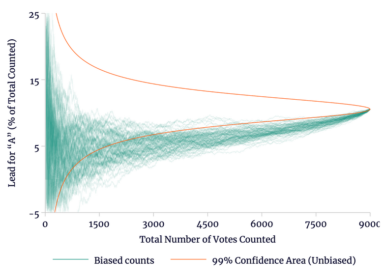
This means that a partial biased count will form a poor estimate for the final result. To make this a bit more clear, we re-present these same counts in Figure 4. Unlike Figure 3, however, we now show the growing lead for candidate A as a share of the total votes counted up to that point.
Figure 4
Leads in Biased Counts as Share of Votes Counted
Source: author’s calculations.
In Figure 4, we see that in the end, candidate A has won by 10.56 percent of all votes (4975–4025). Very early, this vote margin varies by a lot, but as the count progresses, the margin stabilizes. After about 3,000 votes have been examined, 99 percent of unbiased counts show candidate A with a lead of 6.7–14.4 percent (or about 200–430 votes). We might expect at that point that the final lead would be the same 6.7–14.4 percent of 9,000 votes, or 600–1,290.
As an unbiased count progresses, such estimates improve. By the time 7,500 ballots have been examined, the lead is around 9.3–11.8 percent, or 700–880 votes. Any individual count may still mislead somewhat, due to bad luck. There is only about a 1 in 10,000 chance that the lead will be 8.8 percent or less by the 7,500 ballot mark (corresponding to 660 votes or less).
The same cannot be said for the biased count. Again, the margin varies quite a lot early, but at nearly every point a biased, partial, count is almost guaranteed to mislead as to the final vote. By the time 3,000 votes have been examined, only 18 of the 100 biased counts show candidate A with a lead of 6.7 percent. Even after 7,500 votes have been counted, A’s lead is below 8.8 percent in 90 of the 100 biased examples.
Just as tending to select nickels before dimes led to an underestimate of the value of the coins in the jar, a small bias against candidate A in selecting ballots leads the partial counts to significantly underestimate overall support for A.
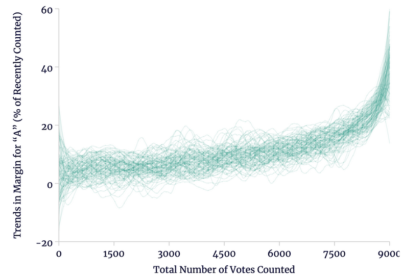
Likewise, when we have a counting bias in favor of B, we will likely observe a sharp increase in support for A late in the count. In Figure 4, the margins were cumulative over the progress of the count. In Figure 5, we see the margins on only recently counted ballots. That is, in Figure 4, the reported margins at “4,500” consider all ballots in the first half of the count while in Figure 5, the reported margins at “4,500” consider only ballots in the very middle of the count.
We see again that candidate A wins by about 4 percentage points on the earliest-counted votes (52–48), increasing to about 13 percentage points (56.5–43.5) for votes 6,000–7,500. In the last sixth of the count, the margin tends to rise much more sharply — to an average of perhaps 36 percentage points (68–32) by the end.
Figure 5
Support for A in Biased Counts Often Shows Sharp Increase Near the End
Source: author’s calculations.
Again, there is nothing unusual about the votes at the end, except that there has been a counting bias throughout. The bias at the end is not greater than the bias at the beginning; rather the cumulative effect of the bias leaves relatively few B votes at the end of the count.
Importantly, this counting bias means not only that later-counted votes on average show more support for A than do early-counted votes, but that the trend usually turns quite sharply in favor of A late in the count. This means that even if we recognize that there was a counting bias, we must not naively assume that the trend in the first half or even first five-sixths of the count will persist. If, after 7,500 votes had been counted, we assumed the trend would continue as a straight line, we would wind up severely underestimating the final margin of victory for A. We may easily understate A’s support by a percentage point or more.
As we will see in this series, the preliminary count in Bolivia’s 2019 presidential election suffered from a similar bias: polling stations favoring the opposition — Carlos Mesa in particular — tended to be counted before polling stations favoring the incumbent, Morales. Nickels before dimes. Escobari and Hoover fail to fully account for this bias and this leads them to underestimate Morales’s lead late in the preliminary count. Consequently, they erroneously infer the existence of widespread fraud. In our next post, we will begin to explore the actual counting biases present in that election.