Article
Escobari and Hoover’s “Difference Estimates” Must Not Be Taken at Face Value

Article
This is the seventh in a series of blog posts addressing a report by Diego Escobari and Gary Hoover covering the 2019 presidential election in Bolivia. Their conclusions do not hold up to scrutiny, as we observe in our report Nickels Before Dimes. Here, we expand upon various claims and conclusions that Escobari and Hoover make in their paper. Links to other posts: part one, part two, part three, part four, part five, part six, part eight, and part nine.
In the previous post, we took note of an error in the margin calculations by Escobari and Hoover. Though the effect on their calculations was small, the incorrect use of Válidos En Acta by Escobari and Hoover (among many others) generated controversy by making it appear that official vote totals did not correctly sum. Rather, these reflect clerical errors made by jurors at individual polling stations. We now pick up where we left off in post #5 when we noted that there was counting bias in the election. Here, we delve into the effects that bias had on the first results produced by Escobari and Hoover.
We begin with their “Difference Estimates,” almost exactly reproduced below. We attribute the discrepancies (indicated in red) to differences in assigning polling stations to precincts — a problem we identified with the first version of their 2019 paper, and that was likely not completely corrected.
Table 1
| CC | MAS | MAS-CC | ||||
|---|---|---|---|---|---|---|
| (1) | (2) | (3) | (4) | (5) | (6) | |
| Variable | ||||||
| SHUTDOWN | -8.286 (0.324) | 7.975 (0.343) | 16.26 (0.653) | 7.243 (0.437) | 6.762 (0.464) | 0.377 (0.194) |
| Constant | 36.86 (0.136) | 46.69 (0.134) | 9.830 (0.266) | 11.28 (0.162) | 11.36 (0.151) | 12.39 (0.063) |
| Fixed Effects[1] | ||||||
| Municipality | 129.6 | |||||
| Locality | 23.49 | |||||
| Precinct | 124.7 | |||||
| Observations | 34,529 | 34,529 | 34,529 | 34,529 | 34,529 | 34,529 |
| R2 | 0.017 | 0.016 | 0.017 | 0.640 | 0.740 | 0.958 |
Source: TSE and author’s calculations.
Notes: Dependent variables are percentages of Válidos En Acta (frequently missing or otherwise misreported on the tally sheets) and not of official valid votes. Standard errors in parentheses are robust. Differences from Escobari and Hoover noted in red.
[1] F-test statistics for fixed effects are not robust.
Note also that the analysis is not weighted by the number of voters at each station. For example, the constant for column 3 indicates the simple average margin for Morales across polling stations included in the TSE announcement was 9.83 percentage points — almost 2 percentage points above the official result at the time. Likewise, Escobari and Hoover’s result implies the simple average margin for Morales across all polling stations was 12.45 percentage points — again nearly 2 percentage points above the official result. This is because in actual elections, overall vote shares are not calculated the way Escobari and Hoover do. In actual elections, it is the vote totals, and not the average margins, that matter. Thus, polling stations with fewer votes have less impact on the final vote than do polling stations with more votes. Ignoring this makes Escobari and Hoover’s results difficult to put in the proper context.
Consider the two-precinct example of Table 2. In the rural precinct, there were 100 valid votes, which Morales won by 40 votes. In the urban precinct, Mesa won by 25 votes out of 250. The simple average margin is (40-10)/2 = 15 percentage points. But overall (taking both stations as a single group) Morales won by 40-25 = 15 votes out of 350, or only 4.3 percentage points.
Table 2
| Voters | Net Votes | Margin | |
|---|---|---|---|
| Rural | 100 | 40 | +40 |
| Urban | 250 | -25 | -10 |
| Combined | 350 | 15 | 4 |
We turn to column 3 of Table 1 above. In Table 3, we present the results of Escobari and Hoover alongside our replication and corrections to ease context. First, we note that our replication (column 2) exactly reproduces the published results (column 1). Second, we see that in employing the correct number of valid voters in the calculation, we have 22 more observations, missing only four polling stations that were annulled. Third, we note that once we weigh polling station data by the number of valid voters (column 4), the “Constant” falls by nearly 2 percentage points. This reflects putting the numbers in their proper context. Morales’s lead (based on the official numbers) at the polling stations included in the TSE announcement was 7.9 percent of the valid vote.
Likewise, in moving from column 3 to column 4, “SHUTDOWN” grows by 0.5, meaning that in giving too much importance to small polling stations, Escobari and Hoover wind up underestimating the increase in support when moving from stations included in the TSE announcement to those outstanding. Taken as a group, Morales’s margin on outstanding polling stations is 7.883+16.77 = 24.65 percentage points, and not 9.843+16.27 = 26.12.
Table 3
| As Published | Replication | Correct Voters | Weighted | |
|---|---|---|---|---|
| (1) | (2) | (3) | (4) | |
| Variable | ||||
| SHUTDOWN | 16.26 (0.653) | 16.26 (0.653) | 16.27 (0.653) | 16.77 (0.663) |
| Constant | 9.830 (0.266) | 9.830 (0.266) | 9.843 (0.266) | 7.883 (0.264) |
| Observations | 34,529 | 34,529 | 34,551 | 34,551 |
| R2 | 0.017 | 0.017 | 0.017 | 0.019 |
There are several ways of interpreting these results. One is to simply say that they measure the amount by which late polling stations more heavily favored Morales, and make no attribution as to the cause. This analysis is merely descriptive.
Another is to say that these results measure the bias in counting opposition polling stations disproportionately early. Perhaps rural stations that happen to favor Morales were simply more likely to be late and were therefore excluded from the TSE announcement — that is, nickels before dimes.
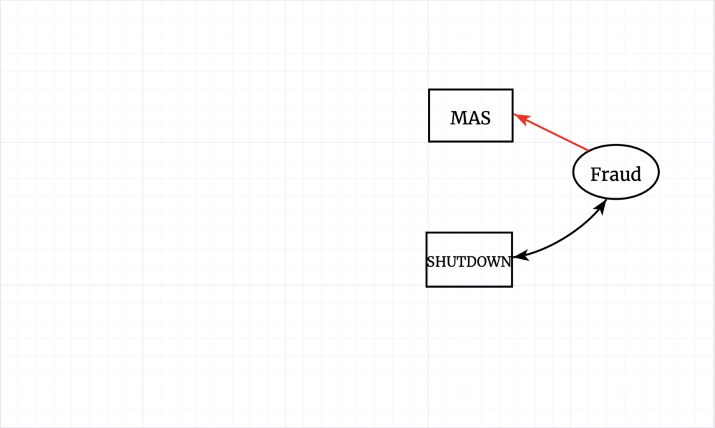
A third is to say that the announcement itself marked a division: the mere fact that a polling station was not included in the announcement explains the increase in support and that if all had been included, Morales would have won by only 7.9 percentage points. Because voting took place before the announcement, exclusion from the announcement should not by itself cause Morales’s support in those polling stations to rise. The implication is that the rise must be due to the addition of fraud, either committed after the announcement or in a deliberate delay in reporting polling station results already known to contain fraud. That is, in this interpretation SHUTDOWN would be a proxy for fraud.
In this figure, we are interested in the connection from fraud to margin, highlighted in red. Fraud is not something we can directly observe in the data, but one proposed mechanism is that the time required to implement fraud required delaying verification of those tally sheets until after the TSE announcement (hence whether or not it was included in the post-announcement “SHUTDOWN” group).
Note that the published result is inconsistent with respect to this interpretation. Escobari and Hoover argue in favor of the 7.9 percentage point counterfactual, but the constant in the model implies a projected margin of 9.8 percentage points — not statistically distinct from the election-determining 10 percentage point threshold. This reinforces our point that the use of weights in the analysis is important when one wishes to interpret the results.
This third explanation of the 16 percentage point difference as a measure of actual fraud is difficult to defend because of the confounding explanations in the second analysis. That is, in the model, SHUTDOWN captures everything impacting Morales’s margin that varies across the groups. There exists a whole apparatus of factors all complicating the interpretation of the 16 percentage point difference as fraud.
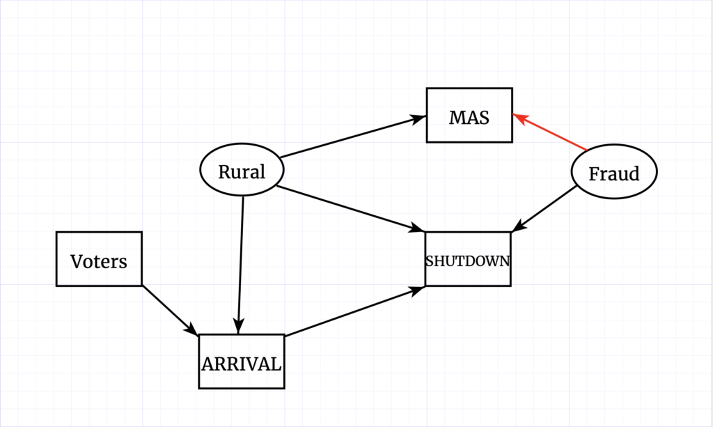
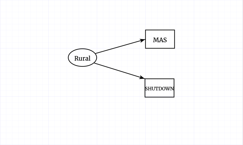
We are still only interested in the effect of fraud indicated in red. Of course, tally sheets wound up in the SHUTDOWN group for benign reasons as well as because of any putative malice. Consider those that transmitted late (late “ARRIVAL” to the electoral authorities) and those that transmitted their transcriptions but could not be verified in a timely manner. We tie both ARRIVAL and SHUTDOWN to rurality, but here “Rural” is a stand-in for a battery of various geographic or socioeconomic factors, any of which may have a different effect on each. Importantly, these same factors carry information about support for Morales, and so impact the observed margin. Finally, the number of voters at any given polling station helps to determine the order of ARRIVAL as smaller stations are able to complete their votes counts more rapidly.
The problem is that if we control for SHUTDOWN alone, that carries with it information about all the geographic factors. For example, given that a station is in the SHUTDOWN group, we can infer that it is more rural and therefore more heavily in favor of Morales. We can’t say if the 16 percentage point difference is all due to the “fraud” Escobari and Hoover seek to measure, or if it is all due to differences in geographic/socioeconomic factors. A more complex statistical model is required.
Of course, it is not easy to quantify — let alone identify — every confounding factor. We must bend somewhat to the reality of data availability. We must recognize that SHUTDOWN is a residual effect. Everything that accounts for the late increase in margin that is not expressly modeled is captured by SHUTDOWN. That includes both possible fraud and any overlooked nickels before dimes. A “statistically significant” SHUTDOWN coefficient doesn’t indicate the existence of fraud, specifically, unless we can adequately disentangle the effects.
To that point, an unexplained 16.77 percentage point difference would be politically worrisome in the absence of other information. Applied to the 16 percent of the election included in the SHUTDOWN group, this implies the exceedingly simple model fails to explain 2.7 percentage points of Morales’s final margin. We can see this directly in the estimated constant of Table 3, Column 4, which says that the non-SHUTDOWN group favored Morales by 7.9 percentage points. If the SHUTDOWN group is effectively identical, then the final election margin should have been close to 7.9 percentage points and not the official 10.56. Thus, the model leaves a politically significant unexplained residual that Escobari and Hoover interpret to be fraud. However, we know for a fact that the critical assumption that the SHUTDOWN group is identical is false. The model does not take into account important differences between the SHUTDOWN and non-SHUTDOWN groups. Nickels before dimes.
One way to cope with a dizzying array of possible differences is to divide polling stations into smaller groups. In doing so, we may hope to make assignments so that within each group these confounding factors are more or less constant — that we cannot easily distinguish one polling station from another except by their inclusion or exclusion from the TSE announcement.
As we will see in the next post, this is the reasoning behind columns 4–6 of Table 1.