Article
Escobari and Hoover Make an Improper Comparison to 2016, Invalidating Their “Difference-in-Difference” Estimates

Article
This is the tenth in a series of blog posts addressing a report by Diego Escobari and Gary Hoover covering the 2019 presidential election in Bolivia. Their conclusions do not hold up to scrutiny, as we observe in our report Nickels Before Dimes. Here, we expand upon various claims and conclusions that Escobari and Hoover make in their paper. Links to posts: part one, part two, part three, part four, part five, part six, part seven, part eight, and part nine.
In the previous post, we observed that even if geography is stable from one election to another, there is no guarantee that the effect of geography on vote shares is consistent over time. This may result in a widening gap between observed margins over the progress of a count, even absent any fraud. We also observed that the results at the polling stations included in the TSE announcement exhibited such a trend. We asserted that this poses a problem for Escobari and Hoover. In this post, we demonstrate how their “difference-in-difference” models mistakenly identify fraud when the difference in trends interacts with the counting bias — even when the resulting trends are linear.
One way of demonstrating this is to apply Escobari and Hoover to synthetic election data where we have total control of the amount of fraud. We may create a “geography” variable. We will not be able to observe this variable directly in our analysis, but it will be constant across precincts and will correlate with ARRIVAL. We may then generate election results based on the hidden geography alone, with no consideration to ARRIVAL. For clarity of illustration, we will then break out the SHUTDOWN group as polling stations in the last sixth of ARRIVAL.
In Figure 1, we see two different synthetic election results. Both the results on the left and the results on the right have the same overall trend over the order in which polling stations transmitted. In each, we have marked out the SHUTDOWN polling stations in green. There is no within-precinct-trend in either the left or right, nor does SHUTDOWN have any impact on the margin. The only difference between left and right is how much geography explains the differences across precincts.
Figure 1
Two Examples of Synthetic Election Data
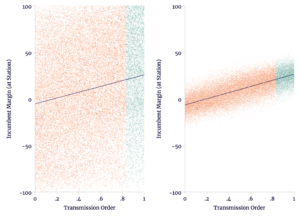
Source: author’s calculations.
On the right, geography explains quite a bit and therefore the overall trend is clearer because the order of transmission is an imperfect proxy for geography.
We may produce difference estimates on this data just as we had on the actual election results of 2019. In both the left and the right, Escobari and Hoover’s difference estimates identify fraud where none exists — unless we adjust at the precinct level.
Table 1
| (1) | (2) | (3) | (4) | |
| SHUTDOWN | 15.46 (0.706) | 0.233 (0.110) | 16.26 (0.141) | 0.132 (0.706) |
| Constant | 7.780 (0.298) | 10.38 (0.037) | 7.370 (0.076) | 10.11 (0.044) |
| Precinct | No | Yes | No | Yes |
| 35,000 | 35,000 | 35,000 | 35,000 | |
| 0.0136 | 0.988 | 0.199 | 0.773 |
Source: author’s calculations.
In generating the synthetic election results, we have not even identified precincts as counted entirely late, so we know there is no late precinct-level fraud. However, that should not stop up from adding in synthetic 2016 data. As we see in Figure 2, the synthetic 2019 results are more sensitive to geography than the 2016 results.
Figure 2
Example of Synthetic Data Covering Multiple Elections
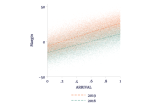
Source: author’s calculations.
So what do Escobari and Hoover do with this added information? In the simple difference models, they simply compared the average margin among those polling stations included in the TSE announcement to those that were excluded. They assume that absent fraud there is no difference between the two. In the “difference-in-difference” models, the baseline for fraud in 2019 is not zero, but whatever difference is observed in 2016. Graphically, we may see Escobari and Hoover’s baseline difference-in-difference model applied to the synthetic data in Figure 3. The thin dashed lines mark the trends for each election and the thick solid lines indicate the model predictions.
Figure 3
Simple Difference-in-Difference Fails on Synthetic Election Data
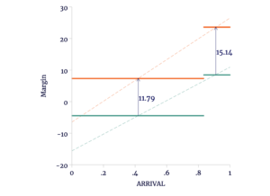
Source: author’s calculations.
Because the trends are not parallel, the average gap between 2016 and 2019 is 11.8 percentage points among polling stations included in the TSE announcement, but 15.1 percentage points among the SHUTDOWN stations. This results in a “difference-in-difference” of 3.3 percentage points (the difference between the late-ARRIVAL difference of 15.1 percentage points and the early-ARRIVAL difference of 11.8 percentage points).
Escobari and Hoover’s interpretation of the 3.3 percentage point double-difference is that there is fraud in the late-ARRIVING polling stations. But there is nothing interesting about these at all, except that they are “geographically” more favorable to the incumbent. The double-difference arises because the margins are more sensitive to geography in 2019 — something that exists throughout the data.
We may, as before, include geographic controls by adjusting at the precinct level. While this will remove the overall trend across elections, it will preserve the cross-election differences; the difference in trends will not change. This means that the difference-in-difference also will not change, and therefore Escobari and Hoover would again misinterpret this increased geographic sensitivity as “fraud.”
Figure 4
Precinct-Level Adjustment of Synthetic Data Has No Effect on the Estimate
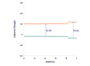
Source: author’s calculations.
In Table 2, we see the statistical output from applying the difference-in-difference model to both the “left” and “right” data and with varying levels of geographic controls. The difference-in-difference is listed as “SHUTDOWN x Y2019.”
Table 2
| (1) | (2) | (3) | (4) | (5) | (6) | |
| SHUTDOWN x Y2019 | 4.703 (1.03) | 4.703 (1.069) | 4.703 (1.456) | 3.343 (0.150) | 3.343 (0.156) | 3.343 (0.212) |
| SHUTDOWN | 10.75 (0.784) | -2.202 (0.543) | 12.91 (0.137) | -1.687 (0.127) | ||
| Y2019 | 11.74 (0.437) | 11.74 (0.436) | 11.74 (0.618) | 11.79 (0.063) | 11.79 (0.065) | 11.79 (0.089) |
| Constant | -3.963 (0.331) | -1.754 (0.229) | -2.129 (0.280) | -4.442 (0.068) | -1.956 (0.047) | -2.241 (0.040) |
| Precinct | No | Yes | Yes | No | Yes | Yes |
| Tally Sheet | No | No | Yes | No | No | Yes |
| 70,000 | 70,000 | 70,000 | 70,000 | 70,000 | 70,000 | |
| 0.0231 | 0.523 | 0.530 | 0.332 | 0.746 | 0.861 | |
Source: author’s calculations.
Note that within each data set, the level of geographic control does not change the point estimate of the double-difference at all, but the uncertainty is greater in the “left” data — which is less fully explained by geography.
The reason that the point estimates are constant within each data set is that our data is complete: we have data for 2016 and 2019 at each polling station. The difference-in-difference model applied to the vote margins reduces exactly to an ordinary difference model applied to the increases in margins from 2016 to 2019. In other words, with the difference-in-difference model we are asking simply by how much more margins rose on average in the SHUTDOWN group compared to the rise in the earlier polling stations. If there is any benign reason why the SHUTDOWN margins would rise by more, then the double-difference overestimates fraud.
There is no fraud in the synthetic data. Rather, the identifying “parallel trends” assumption does not hold. The interpretation of the double-difference as fraud is entirely mistaken.
In the next post, we will apply these methods to the actual election data and observe that the problem of nonparallel trends persists.