Article
Red Herrings: Escobari and Hoover’s Geographic Controls and Common Trends Add Nothing

Article
This is the eleventh in a series of blog posts addressing a report by Diego Escobari and Gary Hoover covering the 2019 presidential election in Bolivia. Their conclusions do not hold up to scrutiny, as we observe in our report Nickels Before Dimes. Here, we expand upon various claims and conclusions that Escobari and Hoover make in their paper. Links to posts: part one, part two, part three, part four, part five, part six, part seven, part eight, part nine, and part ten.
Earlier, we observed that even if geography is stable from one election to another, there is no guarantee that the effect of geography on vote shares is consistent over time. There are completely ordinary and utterly plausible explanations for why election results would be more or less sensitive to geography from one election to another. This may result in a widening gap between observed margins over the progress of a count even absent any fraud
In the last post, we saw the effect this had on Escobari and Hoover’s “difference-in-difference” models. Specifically, the absence of fraud does not guarantee that the identifying “parallel trends” assumption holds. This causes Escobari and Hoover’s approach to mistakenly find fraud where none exists.
Unfortunately, we also observed that we have reason to believe that the parallel trends assumption does not hold in the official data, either. For example, Morales lost support relative to 2016 outside rural areas of Bolivia, and rural areas tended to be counted late. Thus, his loss shrank as rurality of the vote increased. Mesa’s support among opposition voters was disproportionately concentrated in the capital cities. These tended to report early, meaning Morales’s margin further increased over the count. As a consequence, there was an observable, preexisting widening of the differences between 2016 and 2019 over the count at the time of the TSE announcement. There is every reason to expect that the SHUTDOWN polling stations would on average show a bigger increase in Morales’s margin than the stations included in the announcement.
In Figure 1, we see the application of the difference-in-difference models to the official results.
Figure 1
Difference-in-Difference Model Applied to Official and Adjusted Results
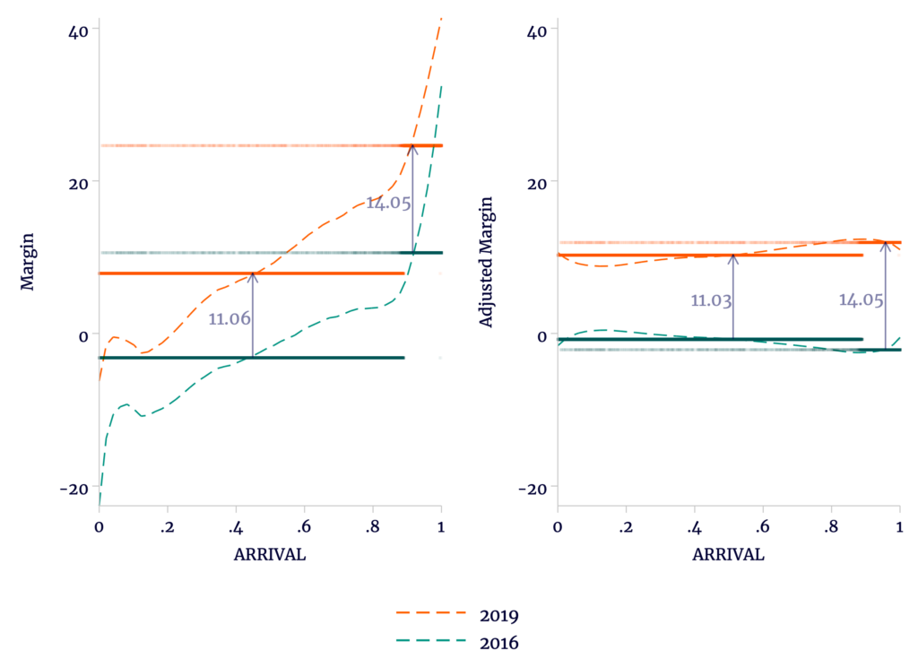
Sources: TSE, OEP, and author’s calculations.
Whether or not we adjust the data by precinct, there is a double-difference of 3 percentage points. However, it seems clear that the trends are not parallel. It is particularly clear in the adjusted data on the right that among polling stations included in the TSE announcement, later reporters have a wider gap between 2016 and 2019 than those polling stations reporting earlier. It is clearly wrong to simply assume that the post-announcement stations, which are largely those that reported even later, should not show a gap at least as wide.
Table 1
Application of Escobari and Hoover’s “Difference-in-Difference Estimates” to Actual Data
|
As Published |
Replication |
|||||
|
(1) |
(2) |
(3) |
(4) |
(5) |
(6) |
|
|
Variable |
||||||
|
SHUTDOWN x Y2019 |
2.964 (0.334) |
2.699 (0.335) |
2.842 (0.459) |
2.996 (0.251) |
3.018 (0.261) |
3.018 (0.355) |
|
SHUTDOWN |
13.30 (0.610) |
-1.090 (0.212) |
13.77 (0.624) |
-1.37 (0.122) |
||
|
Y2019 |
11.99 (0.635) |
11.15 (0.443) |
11.13 (0.612) |
11.06 (0.091) |
11.03 (0.095) |
11.03 (0.129) |
|
Constant |
-2.157 (3.380) |
0.616 (0.298) |
0.438 (0.290) |
-3.173 (0.238) |
-0.742 (0.038) |
-0.960 (0.060) |
|
Fixed Effects |
||||||
|
Precinct |
Yes |
Yes |
||||
|
Station |
Yes |
Yes |
||||
|
Observations |
66,535 |
66,535 |
66,535 |
69,082 |
69,082 |
69,082 |
|
R2 |
0.035 |
0.934 |
0.965 |
0.035 |
0.956 |
0.967 |
Sources: TSE, OEP, and author’s calculations.
Escobari and Hoover next expand their model to include ARRIVAL as a variable — in effect allowing for a trend common to both 2016 and 2019. Because the double-difference is driven by a widening difference between elections, this has no effect on the double-difference. We compare the two unadjusted difference-in-difference models in Figure 2. On the right, we see that the 2016 margins rise more slowly than the common trend, while the 2019 margins rise more quickly.
Figure 2
Allowing an Election-Wide Trend Does Not Change the Double-Difference
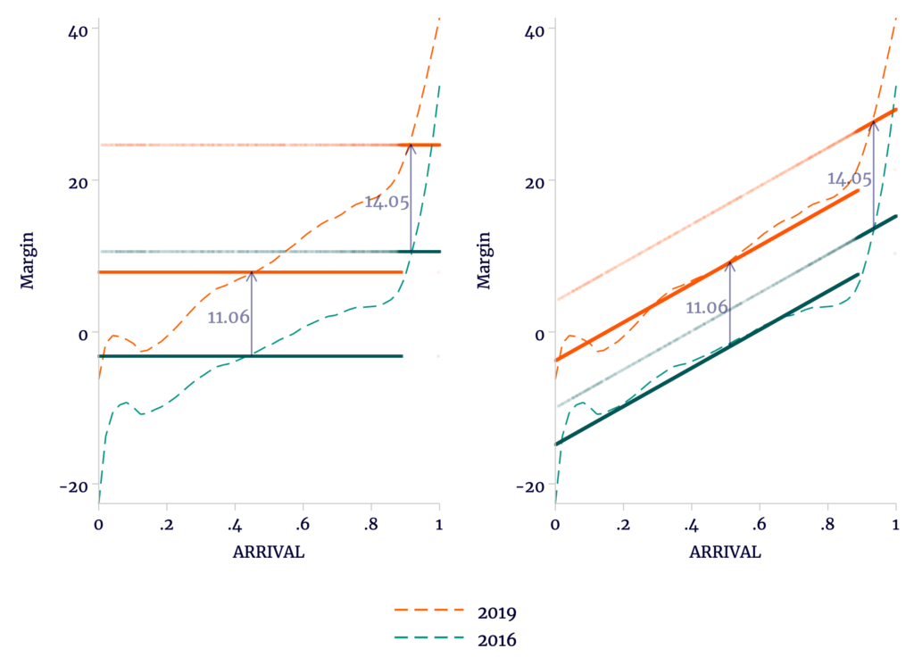
In Table 2, we see the model results including the common trend. In columns 1 and 4, we include the results without trend as reference. Column 5 shows the application with no geographic adjustment. Columns 6 and 7 are replications of the results with geographic effects seen in columns 2 and 3. Taken at face value, and accepting the interpretation of the result as fraud, these effects are not large enough to suggest a reversal of Morales’s first-round victory: 3 percentage points applied to 16 percent of the election comes to less than half of 1 percentage point. However, the nonparallel trends suggest that these estimates are in any case inflated.
Table 2
Application of Escobari and Hoover’s Common-Trend Difference-in-Difference Estimates
|
As Published |
Replication |
||||||
|
(1) |
(2) |
(3) |
(4) |
(5) |
(6) |
(7) |
|
|
Variable |
|||||||
|
SHUTDOWN x Y2019 |
2.964 (0.334) |
2.954 (0.433) |
-2.761 (0.967) |
2.996 (0.251) |
2.992 (0.251) |
3.018 (0.261) |
-3.027 (1.109) |
|
SHUTDOWN |
13.30 (0.610) |
-1.577 (0.262) |
13.77 (0.624) |
4.858 (0.696) |
-1.560 (0.126) |
||
|
Y2019 |
11.99 (0.635) |
11.15 (0.443) |
11.14 (0.611) |
11.06 (0.091) |
11.06 (0.091) |
11.03 (0.095) |
11.03 (0.129) |
|
ARRIVAL |
1.340 (0.242) |
25.26 (0.939) |
0.906 (0.160) |
||||
|
ARRIVAL x SHUTDOWN x Y2019 |
7.277 (1.588) |
7.429 (1.315) |
|||||
|
Constant |
-2.157 (3.380) |
-0.831 (0.311) |
0.198 (0.280) |
-3.173 (0.238) |
-14.81 (0.493) |
-1.179 (0.086) |
-0.960 (0.060) |
|
Fixed Effects |
|||||||
|
Precinct |
Yes |
Yes |
|||||
|
Station |
Yes |
Yes |
|||||
|
Observations |
66,535 |
65,811 |
65,811 |
69,082 |
69,082 |
69,082 |
69,082 |
|
R2 |
0.035 |
0.937 |
0.966 |
0.035 |
0.055 |
0.956 |
0.967 |
Eventually, Escobari and Hoover acknowledge that the trends in the early arrivals differ across years. We explore these models in the next post.